To explore realistic graphics rendering, I have written two Haskell modules on two different techniques that are used in graphics to achieve realism. The first project is a small lighting implementation using a latitude longitude map, the second one is an implementation of the median cut algorithm. The latter is used to deterministically sample an environment map.
A latitude longitude map is a 360 degree image which captures the lighting environments
* Mirror Ball
To use a latitude longitude map when lighting a sphere in the environment, the reflection vector at every point on the sphere is used to get it’s colour. As a simplification, the sphere is assumed to be a perfect mirror, so that one reflection vector is enough to get the right colour.
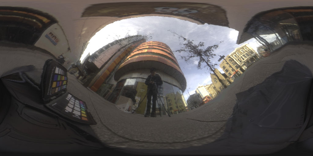
Figure 1: Figure 1: Urban latitude and longitude map.
The latitude longitude map was created by taking a photo of a mirror ball and mapping the spherical coordinates to a rectangle.

Figure 2: Figure 2: Normals calculated on a sphere.
The first step is to calculate the normals at every pixel using the position and size of the sphere. These can be visualised by setting the RGB to the XYZ of the normal at the pixel.
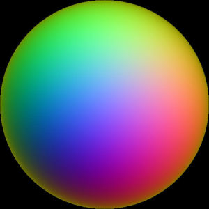
Figure 3: Figure 3: Reflection vectors calculated on a sphere.
The reflection vector can then be calculated and visualised in the same way, by using the following formula: \(r = 2 (n \cdot v) n - v\).
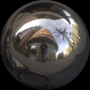
Figure 4: Figure 4: Final image after indexing into the latitude longitude map using reflection vectors.
The reflection vector can be converted to spherical coordinates, which can in turn be used to index into the lat-long map. The colour at the indexed pixel is then set to the position that has that normal.
* Median Cut
The median cut algorithm is a method to deterministically sample an environment map. This is achieved by splitting the environment map along the longest dimension so that there is equal energy in both halves. This is repeated n times recursively in each partition. Once there have been n iterations, the lights are placed in the centroid of each region. Below is an example with 6 splits, meaning there are 2^6 = 64 partitions.
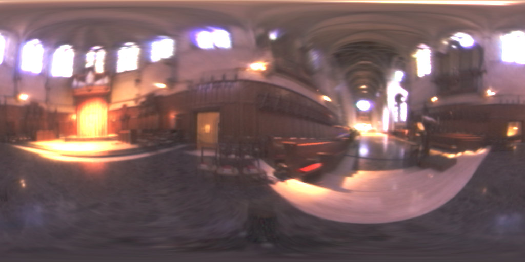
Figure 5: Figure 5: Latitude longitude map of the Grace cathedral.
The average colour of each region is assigned to each light source that was created in each region.
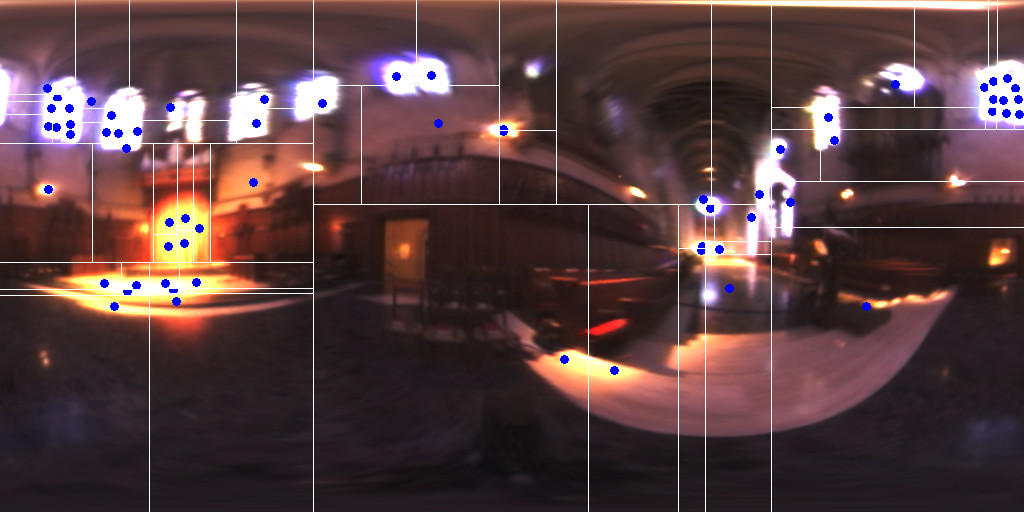
Figure 6: Figure 6: After running the median cut algorithm for 6 iterations.
Finally, these discrete lights can be used to light diffuse objects efficiently, by only having to sample a few lights.
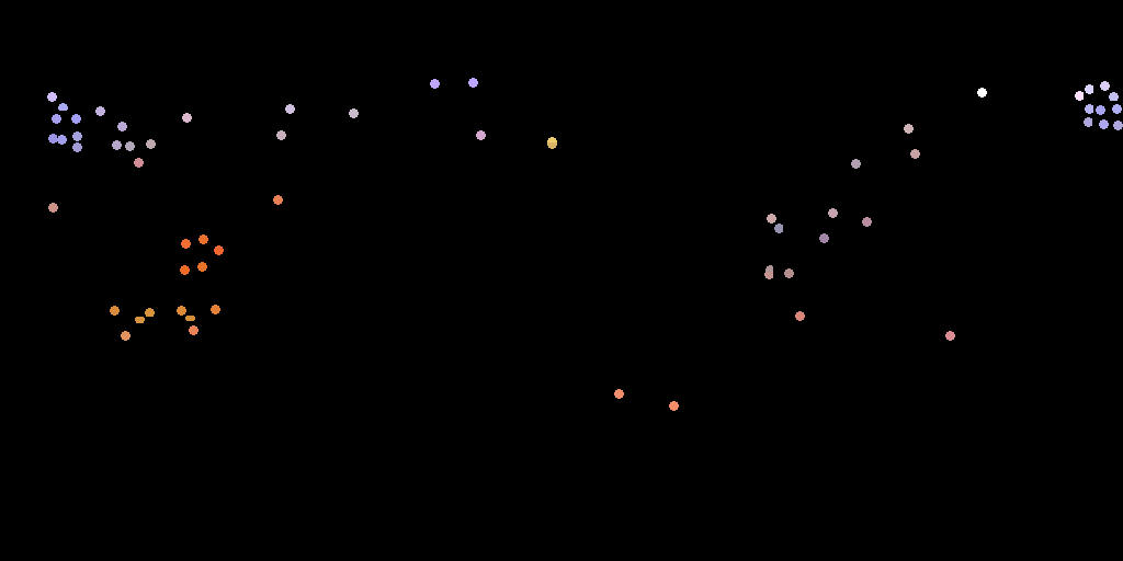
Figure 7: Figure 7: The radiance at each individual sample.